The Backing Predictor (BPD)
When the Next-Line Predictor (NLP) is predicting well, the processor’s Back-end is provided an unbroken stream of instructions to execute. The NLP is able to provide fast, single-cycle predictions by being expensive (in terms of both area and power), very small (only a few dozen branches can be remembered), and very simple (the Bi-Modal Table (BIM) hysteresis bits are not able to learn very complicated or long history patterns).
To capture more branches and more complicated branching behaviors, BOOM provides support for a Backing Predictor (BPD).
The BPD ‘s goal is to provide very high accuracy in a (hopefully) dense area. The BPD only makes taken/not-taken predictions; it therefore relies on some other agent to provide information on what instructions are branches and what their targets are. The BPD can either use the BTB for this information or it can wait and decode the instructions themselves once they have been fetched from the i-cache. This saves on needing to store the PC tags and branch targets within the BPD [7].
The BPD is accessed throughout the Fetch stages and in parallel with the instruction cache access and BTB (see Fig. 8). This allows the BPD to be stored in sequential memory (i.e., SRAM instead of flip-flops). With some clever architecting, the BPD can be stored in single-ported SRAM to achieve the density desired.

Fig. 8 The BOOM Front-end. Here you can see the BTB and Branch Predictor on the lower portion of the diagram. The instructions returning from the instruction cache are quickly decoded; any branches that are predicted as taken from the BTB or Backing Predictor (BPD) will redirect the Front-end from the F4 stage. Prediction snapshots and metadata are stored in the Branch Rename Snapshots (for fixing the predictor after mispredictions) and the Fetch Target Queue (FTQ) (for updating the predictors in the Commit stage).
Making Predictions
When making a prediction, the BPD must provide the following:
- is a prediction being made?
- a bit-vector of taken/not-taken predictions
As per the first bullet-point, the BPD may decide to not make a prediction. This may be because the predictor uses tags to inform whether its prediction is valid or there may be a structural hazard that prevented a prediction from being made.
The BPD provides a bit-vector of taken/not-taken predictions, the size of the bit-vector matching the Fetch Width of the pipeline (one bit for each instruction in the Fetch Packet ). A later Fetch stage will will decode the instructions in the Fetch Packet , compute the branch targets, and decide in conjunction with the BPD ‘s prediction bit-vector if a Front-end redirect should be made.
Jump and Jump-Register Instructions
The BPD makes predictions only on the direction (taken versus not-taken) of conditional branches. Non-conditional “jumps” (JAL) and “jump-register” (JALR) instructions are handled separately from the BPD . [8]
The NLP learns any “taken” instruction’s PC and target PC - thus, the NLP is able to predict jumps and jump-register instructions.
If the NLP does not make a prediction on a JAL instruction, the pipeline will redirect the Front-end in F4 (see Fig. 5). [9]
Jump-register instructions that were not predicted by the NLP will be sent down the pipeline with no prediction made. As JALR instructions require reading the register file to deduce the jump target, there’s nothing that can be done if the NLP does not make a prediction.
Updating the Backing Predictor
Generally speaking, the BPD is updated during the Commit stage. This prevents the BPD from being polluted by wrong-path information. [10] However, as the BPD makes use of global history, this history must be reset whenever the Front-end is redirected. Thus, the BPD must also be (partially) updated during Execute when a misprediction occurs to reset any speculative updates that had occurred during the Fetch stages.
When making a prediction, the BPD passes to the pipeline a “response info packet”. This “info packet” is stored in the Fetch Target Queue (FTQ) until commit time. [11] Once all of the instructions corresponding to the “info packet” is committed, the “info packet” is set to the BPD (along with the eventual outcome of the branches) and the BPD is updated. The Fetch Target Queue (FTQ) for Predictions covers the FTQ , which handles the snapshot information needed for update the predictor during Commit. Rename Snapshot State covers the Branch Rename Snapshots , which handles the snapshot information needed to update the predictor during a misspeculation in the Execute stage.
Managing the Global History Register (GHR)
The Global History Register (GHR) is an important piece of a branch
predictor. It contains the outcomes of the previous N branches (where
N is the size of the GHR ). [12]
When fetching branch i, it is important that the direction of the
previous i-N branches is available so an accurate prediction can be
made. Waiting until the Commit stage to update the GHR
would be too late (dozens of branches would be inflight and not
reflected!). Therefore, the GHR must be updated
speculatively, once the branch is fetched and predicted.
If a misprediction occurs, the GHR must be reset and updated to reflect the actual history. This means that each branch (more accurately, each Fetch Packet ) must snapshot the GHR in case of a misprediction. [13]
There is one final wrinkle - exceptional pipeline behavior. While each branch contains a snapshot of the GHR , any instruction can potential throw an exception that will cause a Front-end redirect. Such an event will cause the GHR to become corrupted. For exceptions, this may seem acceptable - exceptions should be rare and the trap handlers will cause a pollution of the GHR anyways (from the point of view of the user code). However, some exceptional events include “pipeline replays” - events where an instruction causes a pipeline flush and the instruction is refetched and re-executed. [14] For this reason, a commit copy of the GHR is also maintained by the BPD and reset on any sort of pipeline flush event.
The Fetch Target Queue (FTQ) for Predictions
The Reorder Buffer (see The Reorder Buffer (ROB) and the Dispatch Stage ) maintains a record of all inflight instructions. Likewise, the FTQ maintains a record of all inflight branch predictions and PC information. These two structures are decoupled as FTQ entries are incredibly expensive and not all ROB entries will contain a branch instruction. As only roughly one in every six instructions is a branch, the FTQ can be made to have fewer entries than the ROB to leverage additional savings.
Each FTQ entry corresponds to one Fetch cycle. For each prediction made, the branch predictor packs up data that it will need later to perform an update. For example, a branch predictor will want to remember what index a prediction came from so it can update the counters at that index later. This data is stored in the FTQ .
When the last instruction in a Fetch Packet is committed, the FTQ entry is deallocated and returned to the branch predictor. Using the data stored in the FTQ entry, the branch predictor can perform any desired updates to its prediction state.
There are a number of reasons to update the branch predictor after Commit. It is crucial that the predictor only learns correct information. In a data cache, memory fetched from a wrong path execution may eventually become useful when later executions go to a different path. But for a branch predictor, wrong path updates encode information that is pure pollution – it takes up useful entries by storing information that is not useful and will never be useful. Even if later iterations do take a different path, the history that got it there will be different. And finally, while caches are fully tagged, branch predictors use partial tags (if any) and thus suffer from deconstructive aliasing.
Of course, the latency between Fetch and Commit is inconvenient and can cause extra branch mispredictions to occur if multiple loop iterations are inflight. However, the FTQ could be used to bypass branch predictions to mitigate this issue. Currently, this bypass behavior is not supported in BOOM.
Rename Snapshot State
The FTQ holds branch predictor data that will be needed to update the branch predictor during Commit (for both correct and incorrect predictions). However, there is additional state needed for when the branch predictor makes an incorrect prediction and must be updated immediately. For example, if a misprediction occurs, the speculatively-updated GHR must be reset to the correct value before the processor can begin fetching (and predicting) again.
This state can be very expensive but it can be deallocated once the branch is resolved in the Execute stage. Therefore, the state is stored in parallel with the Branch Rename Snapshot s. During Decode and Rename, a Branch Tag is allocated to each branch and a snapshot of the rename tables are made to facilitate single-cycle rollback if a misprediction occurs. Like the branch tag and Rename Map Table snapshots, the corresponding Branch Rename Snapshot can be deallocated once the branch is resolved by the Branch Unit in Execute.

Fig. 9 The Branch Predictor Pipeline. Although a simple diagram, this helps show the I/O within the Branch Prediction
Pipeline. The Front-end sends the “next PC” (shown as req) to the pipeline in the F0 stage. Within the “Abstract Predictor”,
hashing is managed by the “Abstract Predictor” wrapper. The “Abstract Predictor” then returns a Backing Predictor (BPD) response
or in other words a prediction for each instruction in the Fetch Packet .
The Abstract Branch Predictor Class
To facilitate exploring different global history-based BPD designs, an abstract “BrPredictor” class is provided. It provides a standard interface into the BPD and the control logic for managing the global history register. This abstract class can be found in Fig. 9 labeled “Abstract Predictor”. For a more detailed view of the predictor with an example look at Fig. 12.
Global History
As discussed in Managing the Global History Register, global history is a vital
piece of any branch predictor. As such, it is handled by the abstract
BranchPredictor class. Any branch predictor extending the abstract
BranchPredictor class gets access to global history without having to
handle snapshotting, updating, and bypassing.
Operating System-aware Global Histories
Although the data on its benefits are preliminary, BOOM does support OS-aware global histories. The normal global history tracks all instructions from all privilege levels. A second user-only global history tracks only user-level instructions.
The Two-bit Counter Tables
The basic building block of most branch predictors is the “Two-bit Counter Table” (2BC). As a particular branch is repeatedly taken, the counter saturates upwards to the max value 3 (0b11) or strongly taken. Likewise, repeatedly not-taken branches saturate towards zero (0b00). The high-order bit specifies the prediction and the low-order bit specifies the hysteresis (how “strong” the prediction is).
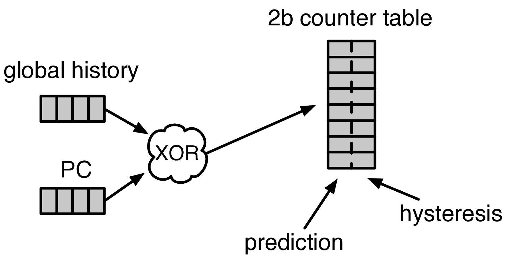
Fig. 10 A GShare Predictor uses the global history hashed with the PC to index into a table of 2-bit counters (2BCs). The high-order bit makes the prediction.
These two-bit counters are aggregated into a table. Ideally, a good branch predictor knows which counter to index to make the best prediction. However, to fit these two-bit counters into dense SRAM, a change is made to the 2BC finite state machine – mispredictions made in the weakly not-taken state move the 2BC into the strongly taken state (and vice versa for weakly taken being mispredicted). The FSM behavior is shown in Fig. 11.
Although it’s no longer strictly a “counter”, this change allows us to separate out the read and write requirements on the prediction and hystersis bits and place them in separate sequential memory tables. In hardware, the 2BC table can be implemented as follows:
The P-bit:
- Read - every cycle to make a prediction
- Write - only when a misprediction occurred (the value of the h-bit).
The H-bit:
- Read - only when a misprediction occurred.
- Write - when a branch is resolved (write the direction the branch took).

Fig. 11 The Two-bit Counter (2BC) State Machine
By breaking the high-order p-bit and the low-order h-bit apart, we can place each in 1 read/1 write SRAM. A few more assumptions can help us do even better. Mispredictions are rare and branch resolutions are not necessarily occurring on every cycle. Also, writes can be delayed or even dropped altogether. Therefore, the h-table can be implemented using a single 1rw-ported SRAM by queueing writes up and draining them when a read is not being performed. Likewise, the p-table can be implemented in 1rw-ported SRAM by banking it – buffer writes and drain when there is not a read conflict.
A final note: SRAMs are not happy with a “tall and skinny” aspect ratio that the 2BC tables require. However, the solution is simple – tall and skinny can be trivially transformed into a rectangular memory structure. The high-order bits of the index can correspond to the SRAM row and the low-order bits can be used to mux out the specific bits from within the row.
The GShare Predictor
GShare is a simple but very effective branch predictor. Predictions are made by hashing the instruction address and the GHR (typically a simple XOR) and then indexing into a table of two-bit counters. Fig. 10 shows the logical architecture and Fig. 12 shows the physical implementation and structure of the GShare predictor. Note that the prediction begins in the F0 stage when the requesting address is sent to the predictor but that the prediction is made later in the F3 stage once the instructions have returned from the instruction cache and the prediction state has been read out of the GShare’s p-table.

Fig. 12 The GShare Predictor Pipeline
The TAGE Predictor
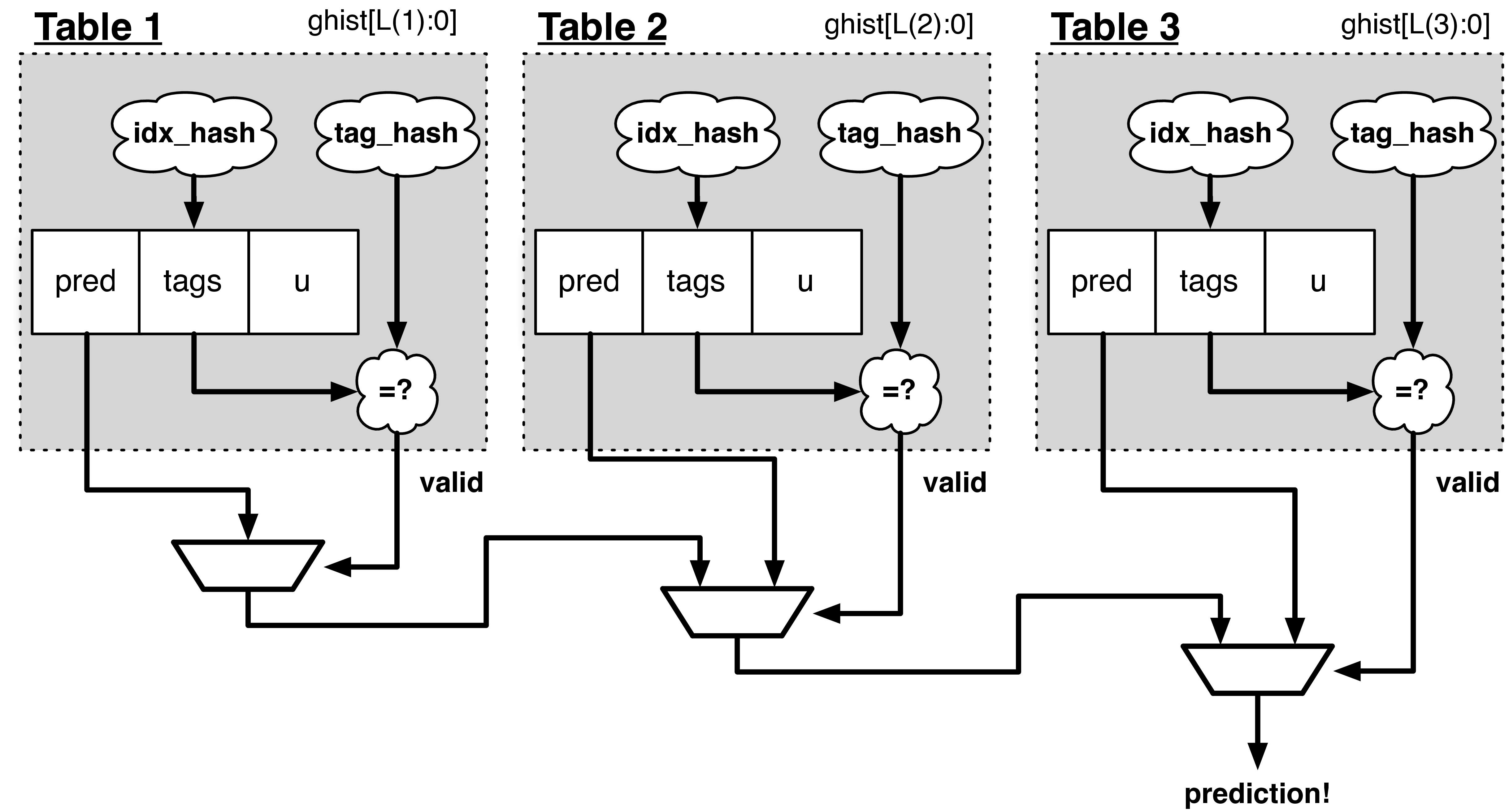
Fig. 13 The TAGE predictor. The requesting address (PC) and the global history are fed into each table’s index hash and tag hash. Each table provides its own prediction (or no prediction) and the table with the longest history wins.
BOOM also implements the TAGE conditional branch predictor. TAGE is a highly-parameterizable, state-of-the-art global history predictor. The design is able to maintain a high degree of accuracy while scaling from very small predictor sizes to very large predictor sizes. It is fast to learn short histories while also able to learn very, very long histories (over a thousand branches of history).
TAGE (TAgged GEometric) is implemented as a collection of predictor tables. Each table entry contains a prediction counter, a usefulness counter, and a tag. The prediction counter provides the prediction (and maintains some hysteresis as to how strongly biased the prediction is towards taken or not-taken). The usefulness counter tracks how useful the particular entry has been in the past for providing correct predictions. The tag allows the table to only make a prediction if there is a tag match for the particular requesting instruction address and global history.
Each table has a different (and geometrically increasing) amount of history associated with it. Each table’s history is used to hash with the requesting instruction address to produce an index hash and a tag hash. Each table will make its own prediction (or no prediction, if there is no tag match). The table with the longest history making a prediction wins.
On a misprediction, TAGE attempts to allocate a new entry. It will only overwrite an entry that is “not useful” (ubits == 0).
TAGE Global History and the Circular Shift Registers (CSRs) [15]
Each TAGE table has associated with it its own global history (and each table has geometrically more history than the last table). The histories contain many more bits of history that can be used to index a TAGE table; therefore, the history must be “folded” to fit. A table with 1024 entries uses 10 bits to index the table. Therefore, if the table uses 20 bits of global history, the top 10 bits of history are XOR’ed against the bottom 10 bits of history.
Instead of attempting to dynamically fold a very long history register every cycle, the history can be stored in a circular shift register (CSR). The history is stored already folded and only the new history bit and the oldest history bit need to be provided to perform an update. Listing 2 shows an example of how a CSR works.
Example:
  A 12 bit value (0b_0111_1001_1111) folded onto a 5 bit CSR becomes
  (0b_0_0010), which can be found by:


               /-- history[12] (evict bit)
               |
 c[4], c[3], c[2], c[1], c[0]
  |                        ^
  |                        |
  \_______________________/ \---history[0] (newly taken bit)


(c[4] ^ h[ 0] generates the new c[0]).
(c[1] ^ h[12] generates the new c[2]).
Each table must maintain three CSRs. The first CSR is used for
computing the index hash and has a size n=log(num_table_entries). As
a CSR contains the folded history, any periodic history pattern matching
the length of the CSR will XOR to all zeroes (potentially quite common).
For this reason, there are two CSRs for computing the tag hash, one of
width n and the other of width n-1.
For every prediction, all three CSRs (for every table) must be snapshotted and reset if a branch misprediction occurs. Another three commit copies of these CSRs must be maintained to handle pipeline flushes.
Usefulness counters (u-bits)
The “usefulness” of an entry is stored in the u-bit counters. Roughly speaking, if an entry provides a correct prediction, the u-bit counter is incremented. If an entry provides an incorrect prediction, the u-bit counter is decremented. When a misprediction occurs, TAGE attempts to allocate a new entry. To prevent overwriting a useful entry, it will only allocate an entry if the existing entry has a usefulness of zero. However, if an entry allocation fails because all of the potential entries are useful, then all of the potential entries are decremented to potentially make room for an allocation in the future.
To prevent TAGE from filling up with only useful but rarely-used entries, TAGE must provide a scheme for “degrading” the u-bits over time. A number of schemes are available. One option is a timer that periodically degrades the u-bit counters. Another option is to track the number of failed allocations (incrementing on a failed allocation and decremented on a successful allocation). Once the counter has saturated, all u-bits are degraded.
TAGE Snapshot State
For every prediction, all three CSRs (for every table) must be snapshotted and reset if a branch misprediction occurs. TAGE must also remember the index of each table that was checked for a prediction (so the correct entry for each table can be updated later). Finally, TAGE must remember the tag computed for each table – the tags will be needed later if a new entry is to be allocated. [16]
Other Predictors
BOOM provides a number of other predictors that may provide useful.
The Base Only Predictor
The Base Only Predictor uses the BTBs BIM to make a prediction on whether the branch was taken or not.
The Null Predictor
The Null Predictor is used when no BPD predictor is desired. It will always predict “not taken”.
The Random Predictor
The Random Predictor uses an LFSR to randomize both “was a prediction made?” and “which direction each branch in the Fetch Packet should take?”. This is very useful for both torturing-testing BOOM and for providing a worse-case performance baseline for comparing branch predictors.
| [7] | It’s the PC Tag storage and Branch Target storage that makes the BTB within the Next-Line Predictor (NLP) so expensive. |
| [8] | JAL instructions jump to a PC+Immediate location, whereas
JALR instructions jump to a PC+Register[rs1]+Immediate location. |
| [9] | Redirecting the Front-end in the F4 Stage for instructions is trivial, as the instruction can be decoded and its target can be known. |
| [10] | In the data-cache, it can be useful to fetch data from the wrong path - it is possible that future code executions may want to access the data. Worst case, the cache’s effective capacity is reduced. But it can be quite dangerous to add wrong-path information to the Backing Predictor (BPD) - it truly represents a code-path that is never exercised, so the information will never be useful in later code executions. Worst, aliasing is a problem in branch predictors (at most partial tag checks are used) and wrong-path information can create deconstructive aliasing problems that worsens prediction accuracy. Finally, bypassing of the inflight prediction information can occur, eliminating any penalty of not updating the predictor until the Commit stage. |
| [11] | These info packets are not stored in the ROB for two reasons - first, they correspond to Fetch Packet`s, not instructions. Second, they are very expensive and so it is reasonable to size the :term:`Fetch Target Queue (FTQ) to be smaller than the ROB. |
| [12] | Actually, the direction of all conditional branches within a Fetch Packet are compressed (via an OR-reduction) into a single bit, but for this section, it is easier to describe the history register in slightly inaccurate terms. |
| [13] | Notice that there is a delay between beginning to make a prediction in the F0 stage (when the global history is read) and redirecting the Front-end in the F4 stage (when the global history is updated). This results in a “shadow” in which a branch beginning to make a prediction in F0 will not see the branches (or their outcomes) that came a cycle (or two) earlier in the program (that are currently in F1/2/3 stages). It is vitally important though that these “shadow branches” be reflected in the global history snapshot. |
| [14] | An example of a pipeline replay is a memory ordering failure in which a load executed before an older store it depends on and got the wrong data. The only recovery requires flushing the entire pipeline and re-executing the load. |
| [15] | No relation to the Control/Status Registers (CSRs) in RISC-V. |
| [16] | There are ways to mitigate some of these costs, but this margin is too narrow to contain them. |